Maximum Likelihood Estimation

At the core of GraphSLAM is graph optimization - the process of minimizing the error present in all of the constraints in the graph. Let’s take a look at what these constraints look like, and learn to apply a principle called maximum likelihood estimation (MLE) to structure and solve the optimization problem for the graph.

Likelihood

Likelihood is a complementary principle to probability. While probability tries to estimate the outcome given the parameters, likelihood tries to estimate the parameters that best explain the outcome. For example,

Probability: What is the probability of rolling a 2 on a 6-sided die?

(Answer: 1/6)

Likelihood: I’ve rolled a die 100 times, and a 2 was rolled 10% of the time, how many sides does my die have?

(Answer: 10 sides)

When applied to SLAM, likelihood tries to estimate the most likely configuration of state and feature locations given the motion and measurement observations.

Probability & Likelihood Quiz

QUIZ QUESTION: :

To solidify your understanding of the difference between probability and likelihood, label the following problems with their respective terms.

ANSWER CHOICES:

Example	Type of Problem
Probability
Likelihood
Likelihood
Probability
Probability

SOLUTION:

Example	Type of Problem
Probability
Probability
Probability
Likelihood
Likelihood
Likelihood
Likelihood
Probability
Probability
Probability
Probability
Probability
Probability

Feature Measurement Example

Let’s look at a very simple example - one where our robot is taking repeated measurements of a feature in the environment. This example will walk you through the steps required to solve it, which can then be applied to more complicated problems.

The robot’s initial pose has a variance of 0 - simply because this is its start location. Recall that wherever the start location may be - we call it location 0 in our relative map. Every action pose and measurement hereafter will be uncertain. In GraphSLAM, we will continue to make the assumption that motion and measurement data has Gaussian noise.

The robot takes a measurement of a feature, m_1 , and it returns a distance of 1.8 metres.

If we return to our spring analogy - 1.8m is the spring’s resting length. This is the spring’s most desirable length; however, it is possible for the spring to be compressed or elongated to accommodate other forces (constraints) that are acting on the system.

This probability distribution for this measurement can be defined as so,

p(x)=\frac{1}{\sigma\sqrt{2\pi}}e^{-\frac{1}{2}\frac{(z_1-(x_0 + 1.8))^2}{\sigma^2}}

In simpler terms, the probability distribution is highest when z1 and x0 are 1.8 meters apart.

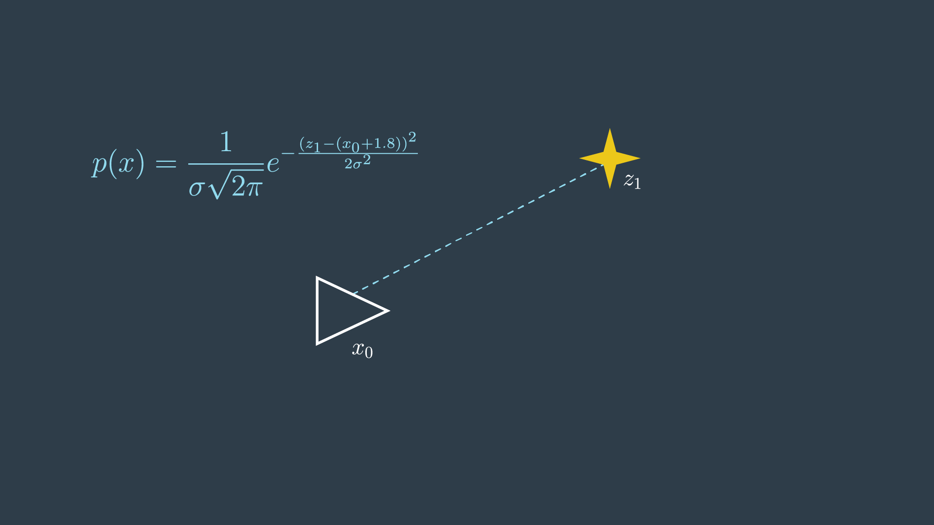
However, since the location of the first pose, x_0 is set to 0, this term can simply be removed from the equation.

p(x)=\frac{1}{\sigma\sqrt{2\pi}}e^{-\frac{1}{2}\frac{(z_1-1.8)^2}{\sigma^2}}

Next, the robot takes another measurement of the same feature in the environment. This time, the data reads 2.2m. With two conflicting measurements, this is now an overdetermined system - as there are more equations than unknowns!

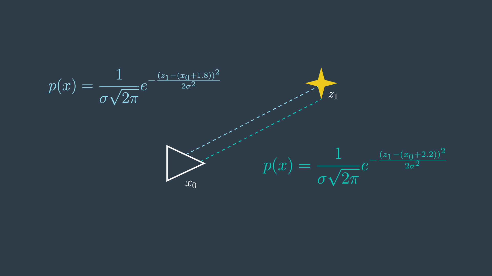
With two measurements, the most probable location of the feature can be represented by the product of the two probabilities.

p(x)=\frac{1}{\sigma\sqrt{2\pi}}e^{-\frac{1}{2}\frac{(z_1 - 1.8)^2}{\sigma^2}} * \frac{1}{\sigma\sqrt{2\pi}}e^{-\frac{1}{2}\frac{(z_1-2.2)^2}{\sigma^2}}

In this trivial example, it is probably quite clear to you that the most likely location of the feature is at the 2.0 meter mark. However, it is valuable to go through the maximum likelihood estimation process to understand the steps entailed, to then be able to apply it to more complicated systems.

To solve this problem analytically, a few steps can be taken to reduce the equations into a simpler form.

Remove Scaling Factors

The value of m that maximizes the equation does not depend on the constants in front of each of the exponentials. These are scaling factors, however in SLAM we are not usually interested in the absolute value of the probabilities, but finding the maximum likelihood estimate. For this reason, the factors can simply be removed.

\color{red}\cancel\frac{1}{\sigma\sqrt{2\pi}}\color{black}e^{-\frac{1}{2}\frac{(z_1 - 1.8)^2}{\sigma^2}} * \color{red}\cancel\frac{1}{\sigma\sqrt{2\pi}}\color{black}e^{-\frac{1}{2}\frac{(z_1- 2.2)^2}{\sigma^2}}

Log-Likelihood

The product of the probabilities has been simplified, but the equation is still rather complicated - with exponentials present. There exists a mathematical property that can be applied here to convert this product of exponentials into the sum of their exponents.

First, we must use the following property, e^ae^b=e^{a+b} , to combine the two exponentials into one.

e^{-\frac{1}{2}\frac{(z_1 - 1.8)^2}{\sigma^2}} * e^{-\frac{1}{2}\frac{(z_1- 2.2)^2}{\sigma^2}}

= e^{-\frac{1}{2}\frac{(z_1 - 1.8)^2}{\sigma^2}-\frac{1}{2}\frac{(z_1- 2.2)^2}{\sigma^2}}

Next, instead of working with the likelihood, we can take its natural logarithm and work with it instead.

ln(e^{-\frac{1}{2}\frac{(z_1 - 1.8)^2}{\sigma^2}-\frac{1}{2}\frac{(z_1- 2.2)^2}{\sigma^2}})

= {-\frac{1}{2}\frac{(z_1 - 1.8)^2}{\sigma^2}-\frac{1}{2}\frac{(z_1- 2.2)^2}{\sigma^2}}

The natural logarithm is a monotonic function - in the log’s case - it is always increasing - as can be seen in the graph below. There can only be a one-to-one mapping of its values. This means that optimizing the logarithm of the likelihood is no different from maximizing the likelihood itself.

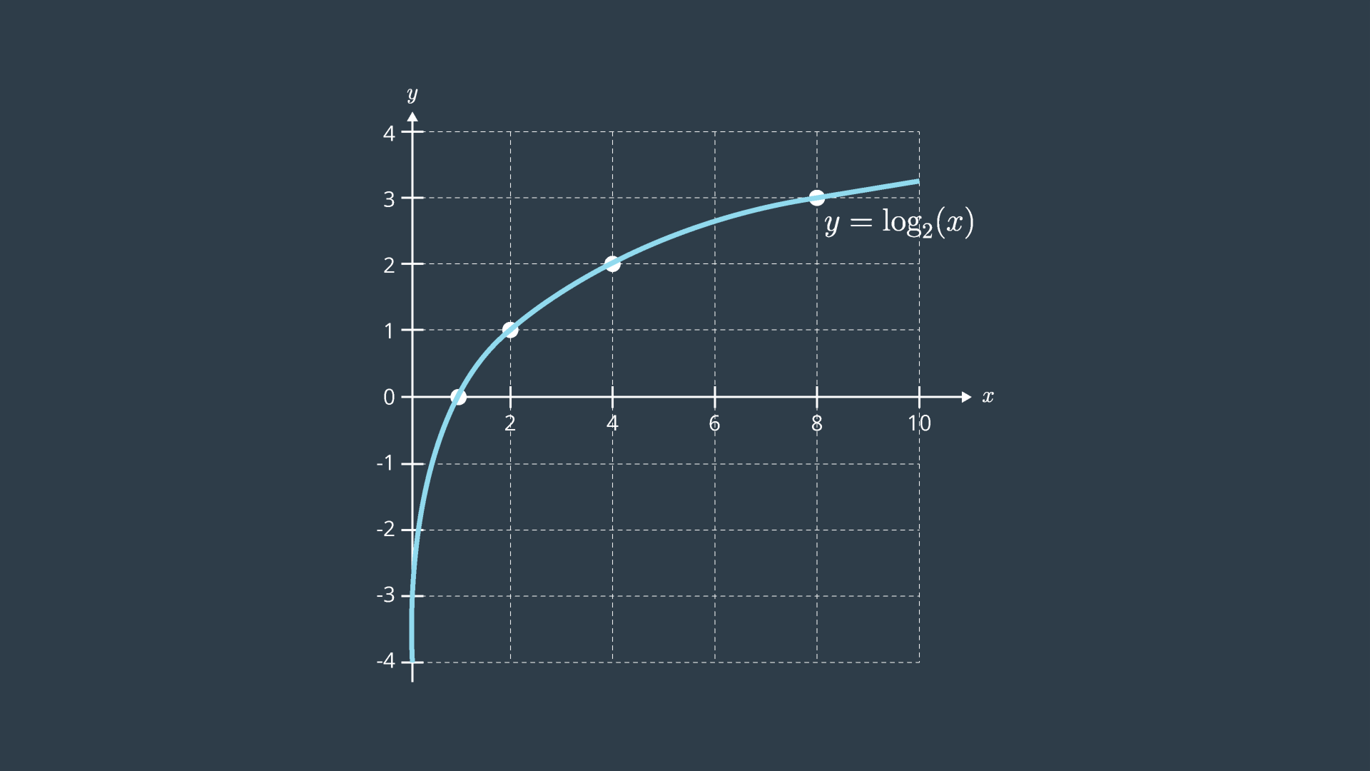
One thing to note when working with logs of likelihoods, is that they are always negative. This is because probabilities assume values between 0 and 1, and the log of any value between 0 and 1 is negative. This can be seen in the graph above. For this reason, when working with log-likelihoods, optimization entails minimizing the negative log-likelihood; whereas in the past, we were trying to maximize the likelihood.

Lastly, as was done before, the constants in front of the equation can be removed without consequence. As well, for the purpose of this example, we will assume that the same sensor was used in obtaining both measurements - and will thus ignore the variance in the equation.

(z_1-1.8)^2+(z_1- 2.2)^2

Optimization

At this point, the equation has been reduced greatly. To get it to its simplest form, all that is left is to multiply out all of the terms.

2z_1^2 - 8z_1 + 8.08

To find the minimum of this equation, you can take the first derivative of the equation and set it to equal 0.

4z_1 - 8 = 0

4z_1 = 8

z_1 = 2

By doing this, you are finding the location on the curve where the slope (or gradient , in multi-dimensional equations) is equal to zero - the trough! This property can be visualized easily by looking at a graph of the error function.

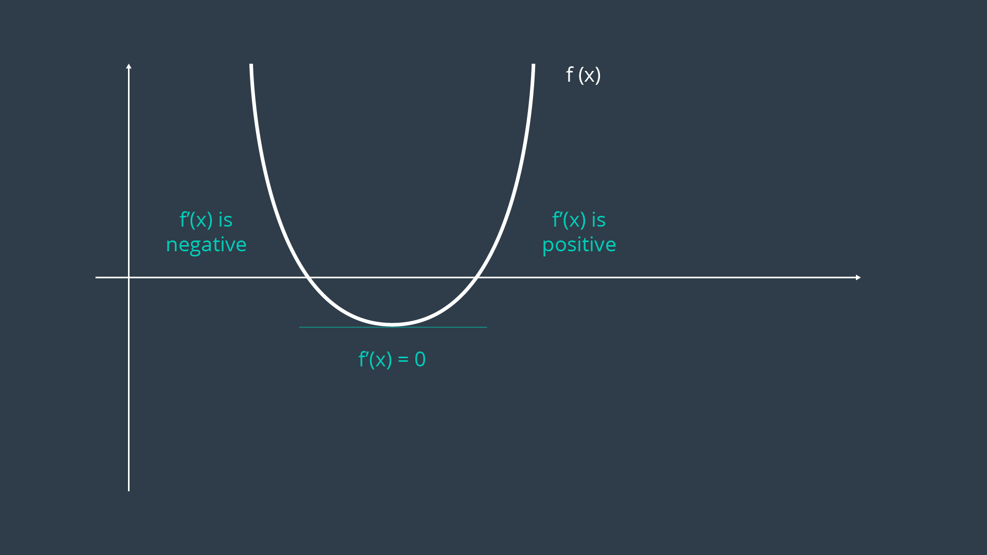
In more complex examples, the curve may be multimodal, or exist over a greater number of dimensions. If the curve is multimodal, it may be unclear whether the locations discovered by the first derivative are in fact troughs, or peaks. In such a case, the second derivative of the function can be taken - which should clarify whether the local feature is a local minimum or maximum.

Overview

The procedure that you executed here is the analytical solution to an MLE problem. The steps included,

Removing inconsequential constants,
Converting the equation from one of likelihood estimation to one of negative log-likelihood estimation , and
Calculating the first derivative of the function and setting it equal to zero to find the extrema.

In GraphSLAM, the first two steps can be applied to every constraint. Thus, any measurement or motion constraint can simply be labelled with its negative log-likelihood error. For a measurement constraint, this would resemble the following,

\frac{(z_t - (x_t + m_t))^2}{\sigma^2}

And for a motion constraint, the following,

\frac{(x_t - (x_{t-1} + u_t))^2}{\sigma^2}

Thus, from now on, constraints will be labelled with their negative log-likelihood error,

with the estimation function trying to minimize the sum of all constraints,

J_{GraphSLAM} = \sum_t\frac{(x_t - (x_{t-1} + u_t))^2}{\sigma^2} + \sum_t\frac{(z_t - (x_t + m_t))^2}{\sigma^2}

In the next section, you will work through a more complicated estimation example to better understand maximum likelihood estimation, since it really is the basis of GraphSLAM.